Statistics
What Is Likelihood in Statistics?
A plain-English guide to likelihood in statistics: how it differs from probability, how maximum likelihood estimation works, and what likelihood ratios mean.
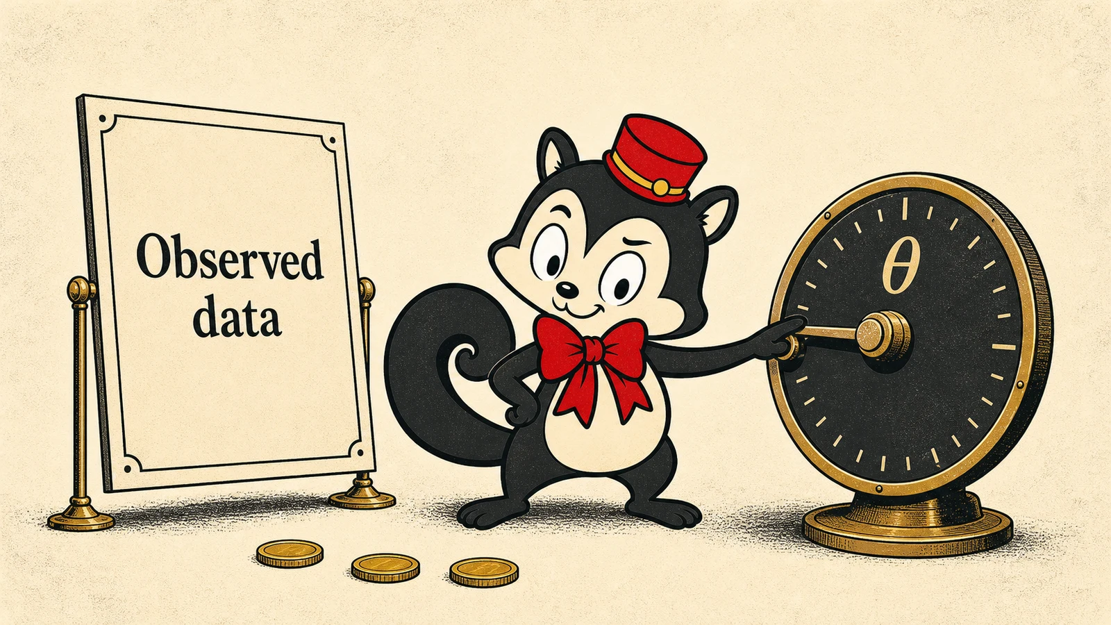
Likelihood is one of those statistical terms that becomes confusing almost immediately.
The formula often looks exactly like a probability formula, but textbooks insist that probability and likelihood are not the same thing. The word itself does not help much either. In ordinary English, likely simply means that something is probable.
The central idea, however, is not as difficult as it first appears.
Likelihood is a function that fixes the data we actually observed and compares how readily different parameter values could have produced it.
The difference between probability and likelihood is not usually the formula itself. It is a difference in what we hold fixed and what we compare.
We will use a coin that produces eight heads in ten tosses to examine probability, maximum likelihood estimation, log-likelihood, and likelihood ratios.
Then, naturally, we will watch black-and-white crime films.
Likelihood vs probability in 30 seconds
Here is the basic picture:
- Probability fixes a model or parameter and asks what data could occur.
- Likelihood fixes the observed data and compares parameter values.
- In , likelihood holds fixed and varies ; probability holds fixed and varies .
- The parameter value with the highest likelihood is the maximum likelihood estimate.
- Likelihood is not the probability that a parameter is correct.
- The absolute value of a likelihood is usually less important than its maximum, shape, or ratio to another likelihood.
- A likelihood ratio compares how readily two hypotheses could have produced the same observed data.
Now let us unpack each part.
The definition of likelihood
Suppose the observed data are , and the model contains an unknown parameter .
A likelihood function is commonly written as
The expression describes how readily data arise when the parameter is .
The important part is that the same expression can be viewed in two different directions.
Viewed as a probability distribution
Fix the parameter , and allow the possible data to vary:
Now we are asking: if the model has this particular setting, what data could occur, and how probable or dense would each result be?
Viewed as a likelihood function
Now fix the data that have already been observed, and vary the parameter :
The question becomes: we have already observed this result. Under which parameter values would it have been most natural?
It is the same mathematical expression, but we are looking along a different axis. [1] [2]
Probability and likelihood: what changes?
| Held fixed | Compared | |
|---|---|---|
| Probability | Model or parameter | Possible data |
| Likelihood | Observed data | Model or parameter |
Imagine a coin whose probability of landing heads is 0.8.
A probability question: If a coin has an 80% chance of landing heads, what is the probability of observing eight heads in ten tosses? Here, is fixed.
A likelihood question: We tossed a coin ten times and observed eight heads. Which value of best fits that result? Now the data are fixed, and we compare possible coins: .
The formula may be the same, but the direction of the question has changed.
With continuous data, likelihood uses density—not point probability
For discrete outcomes, such as heads or tails, can represent the probability of a particular result.
For continuous measurements, such as height or temperature, the probability of observing one exact value is ordinarily zero. In a continuous model, likelihood therefore uses the probability density at the observed value.
- Discrete model: evaluate a probability mass.
- Continuous model: evaluate a probability density.
A density can be greater than 1. This is one reason likelihood values are not generally restricted to the interval from 0 to 1. [1]
A coin example: eight heads in ten tosses
Let be the probability that a coin lands heads. We toss it ten times and observe eight heads and two tails.
If the observed data are the number of heads, the likelihood is
| Probability of heads, p | Likelihood of exactly eight heads |
|---|---|
| 0.5 | 0.044 |
| 0.8 | 0.302 |
| 0.9 | 0.194 |
Among these candidates, has the highest likelihood. A fair coin could still produce eight heads, and a coin with could too. But the split of eight heads and two tails fits 0.8 better than either alternative. This is also the standard binomial MLE pattern illustrated in the UTokyo material. [8]
This statement is correct: if , the probability of observing exactly eight heads in ten tosses is about 30.2%.
This statement is not: after observing eight heads, the probability that is 30.2%.
Try the coin example
Keep the evidence. Turn the dial.
Start with eight heads. Move the coin’s probability of heads to see which values fit that observation. Then change the observed count and watch the peak move.
- Count likelihood, L(p)
- 0.0439
- Relative to the maximum
- 0.146
- Best-fitting p
- 0.8
For 8 heads in ten tosses, the likelihood is highest at p = 0.8. At p = 0.50, the count likelihood is 0.0439, or 0.146 of its maximum.
The numerical value depends on how the data are represented
Above, we treated the data as a count: eight of ten tosses were heads. That gives
If we treat the exact sequence—H, H, H, H, H, H, H, H, T, T—as the data, its likelihood is
The two functions differ by a factor of 45:
But 45 does not depend on . Both functions therefore have the same maximizing value, the same likelihood ratios, and the same maximum likelihood estimate. Multiplying by a positive parameter-independent constant does not change the relative information. [1] [2]
What is maximum likelihood estimation?
Maximum likelihood estimation, usually abbreviated MLE, selects the parameter value that maximizes the likelihood. For our coin, the maximizing value is
We observed heads in eight of ten tosses, so the maximum likelihood estimate of the probability of heads is 0.8. It does not mean that the coin’s true probability must be exactly 0.8. It means that 0.8 makes these observed data most likely within this model.
An MLE is not always unbiased or uniquely defined. In some models an unrestricted maximum may not exist, and familiar large-sample properties require regularity conditions. [2] [3] Fisher’s 1922 paper established the method’s mathematical foundations; its earlier development is reconstructed in Aldrich’s historical account. [4] [5]
Why statisticians use log-likelihood
In practice, statisticians often work with the log-likelihood:
Taking a logarithm does not change the location of the maximum because the logarithm is strictly increasing. Likelihoods often multiply many probabilities or densities:
After taking logs, the product becomes a sum:
Sums are easier to differentiate and easier for computers to handle. They also help avoid numerical underflow when many very small values would otherwise be multiplied together. The log-likelihood is the same likelihood wearing clothes that are easier to calculate in. [2] [4]
Likelihood is not the probability that a parameter is correct
A parameter value with high likelihood fits the observed data well relative to competing values. But likelihood alone does not tell us the probability that this parameter value is true.
Bayesian statistics introduces a prior distribution for the parameter and updates it using the likelihood:
Likelihood is a crucial ingredient of the posterior distribution, but it is not the posterior distribution itself. [2] [4]
An ingredient can be important without being the finished meal. I would not serve flour by itself for dinner.
What is a likelihood ratio?
A likelihood ratio directly compares two parameter values or hypotheses:
In the coin example, compare with :
The observed result of eight heads is about 6.87 times more likely under the model than under . It does not mean that 0.8 is 6.87 times more likely to be true.
To update the odds of two hypotheses in a Bayesian framework, we also need the odds assigned before seeing the data:
A likelihood ratio measures how the data shift the comparison between hypotheses. It does not create the entire comparison from nothing. [2] [6]
Rare evidence is not the same as a high probability of guilt
Likelihood ratios also matter in legal reasoning. Consider these two conditional probabilities:
A common mistake is to reason: if the defendant were innocent, this evidence would be extremely rare; therefore, after seeing the evidence, the probability of innocence must also be extremely small. This reversal is known as the prosecutor’s fallacy. [6] [7]
Rare evidence does not automatically identify one person as guilty. We must consider who else could have produced it, which competing hypotheses are being compared, their plausibility before the evidence, and whether the statistical model represents the situation. A likelihood ratio can describe relative support for two stated hypotheses. It does not directly provide the probability of guilt.
Common misunderstandings about likelihood
1. Likelihood is simply a more difficult word for probability
The formulas may look identical, but probability fixes a model and considers possible data. Likelihood fixes observed data and compares model settings.
2. The parameter with the highest likelihood must be true
The MLE is the value that best fits the observed data within the chosen model. A poor model or limited data may still lead far from the truth.
3. A likelihood of 0.3 means a 30% probability that the parameter is correct
No. In the coin example, 0.302 is the probability of exactly eight heads if . It is not the probability that after seeing the result.
4. Likelihood must lie between 0 and 1
A discrete probability mass lies between 0 and 1, but continuous densities can exceed 1. A likelihood can also be multiplied by a positive parameter-independent constant without changing its maximum or ratios.
5. Set the derivative to zero, and you have automatically found the MLE
A stationary point may be a maximum, minimum, or saddle point. The maximum could also lie at the boundary. You must still examine the second derivative, boundaries, and overall function.
Likelihood in one sentence
Likelihood is a way to fix the observed data and compare how readily different parameter values could have produced them.
Probability looks from a model toward possible data. Likelihood looks from observed data back toward possible model settings. Maximum likelihood estimation selects the parameter value with the highest likelihood. A likelihood ratio compares the relative support that the same data provide to two hypotheses. And likelihood is not the probability that a parameter or hypothesis is true.
Once we begin fixing evidence and comparing competing explanations, we naturally want to watch black-and-white crime films.

Thinking about likelihood through black-and-white films

12 Angry Men
Let us begin with Sidney Lumet’s 12 Angry Men.
A teenage boy is on trial for murder, and twelve jurors enter a single room to decide whether he is guilty. In the first vote, almost everyone is ready to convict him. One juror asks them to slow down and examine the evidence again.
Could the witness really have seen what he claimed to see? Does the stated timeline make sense? Was the alleged murder weapon truly rare enough to point uniquely toward the defendant?
The jurors are largely considering the same evidence, but they disagree about which explanation makes that evidence most coherent.
This is not a film in which anyone calculates a likelihood function.
Still, its structure—refusing to connect evidence directly to a conclusion and reconsidering the same evidence under competing hypotheses—fits beautifully after learning the basic idea of likelihood.
Nearly the entire film takes place in one room, yet the pressure between the jurors, the heat, their prejudices, and their growing uncertainty steadily intensify the tension.
It becomes a vivid way to revisit the relationship between evidence and hypotheses—and even to review the statistical idea without turning the film into a lesson.
Double Indemnity
The black-and-white film most closely connected to the logic of likelihood may be Billy Wilder’s Double Indemnity.
Insurance salesman Walter Neff meets Phyllis Dietrichson and becomes involved in a plan to murder her husband, disguise the death as an accident, and collect the insurance money. They are trying to create an observed event that looks as though it came from the wrong underlying cause.
Then insurance investigator Barton Keyes begins asking whether the apparent accident is really plausible. If this were an ordinary accident, how likely would these particular details be? If it were a planned murder, how well would that hypothesis explain the strange combination of events?
Keyes does not write a likelihood function on a blackboard. But he is comparing the same observed event under two competing explanations—the basic move behind likelihood.
The film offers much more than a statistical connection: dangerous conversations, the tightening pressure of a plan that cannot hold together, lines of shadow cutting across rooms, and the bond between Walter and Keyes. If you watch only one film after learning about likelihood, this is a particularly fitting choice.
The Third Man
Next, try Carol Reed’s The Third Man.
American writer Holly Martins arrives in postwar Vienna after being invited by his old friend Harry Lime. When Holly arrives, he is told that Harry has died in a traffic accident. That is the first explanation.
But as Holly speaks to the people who witnessed the event, the details begin to resist it. How many people carried the body? Who was actually present? Why do the accounts fail to match? Could another hypothesis explain the observed details more naturally than the official story?
Holly wants to believe in the friend he remembers. The evidence gradually begins constructing a different person.
The film also gives us a war-damaged Vienna, wet stone streets, tilted camera angles, deep shadows, underground tunnels, and a strangely playful zither score. After studying likelihood, it may be wise to examine not only the evidence, but also the hypothesis you most want to believe.
Rashomon
Finally, watch Akira Kurosawa’s Rashomon.
A bandit, a samurai’s wife, the dead samurai, and a woodcutter give different accounts of the same event in a forest. A simple likelihood example begins by fixing the observed data. In Rashomon, even that foundation becomes unstable.
What actually happened? Who saw what? How accurately does each testimony represent the event? How does each speaker want to appear?
Before comparing hypotheses, we must ask how the observations themselves were produced. That matters in statistics too. A perfectly calculated likelihood can still lead toward the wrong conclusion if we misunderstand the process that generated the data.
Rashomon is not a statistics lesson. It is a deeply cinematic work built from rain at the ruined gate, shifting sunlight in the forest, and the same event repeatedly returning in a different form. Watching it after learning about likelihood makes the statistical problem more complicated. It makes the film more interesting.
A final summary
Likelihood fixes observed data and compares candidate parameters or hypotheses. Probability fixes a model and asks what data may arise from it. MLE selects the parameter value that maximizes likelihood. Log-likelihood makes calculations easier without changing the maximizing point. Likelihood ratios compare the relative support the data give to competing hypotheses, but likelihood is not the probability that a hypothesis is true.
Choose 12 Angry Men for evidence and the danger of jumping too quickly from observation to conclusion. Choose Double Indemnity for the clearest connection between observed events and competing explanations. Choose The Third Man for the tension between evidence and the hypothesis you want to believe. Choose Rashomon when you are ready to ask whether the data themselves can be trusted.
For another guided path, follow Your first Japanese classic, which begins with Rashomon, or return to the Journal. If you would rather choose by mood than by hypothesis, Ask Momo can narrow the evening down.
References and editorial note
Sources were checked on August 1, 2026. The statistical definitions and cautions above follow the cited academic and professional sources. The explanations, examples, jokes, transition, and film pairings are Monocurator’s editorial work.
- Flávio B. Gonçalves and Pedro Franklin (2021), On the Definition of Likelihood Function, arXiv:1906.10733, version 4.
- Yudi Pawitan (2001), In All Likelihood: Statistical Modelling and Inference Using Likelihood, Oxford University Press, DOI 10.1093/oso/9780198507659.001.0001.
- E. L. Lehmann and George Casella (1998), Theory of Point Estimation, 2nd ed., Springer, DOI 10.1007/b98854.
- R. A. Fisher (1922), “On the Mathematical Foundations of Theoretical Statistics,” Philosophical Transactions of the Royal Society of London, Series A 222, 309–368, DOI 10.1098/rsta.1922.0009.
- John Aldrich (1997), “R. A. Fisher and the Making of Maximum Likelihood 1912–1922,” Statistical Science 12(3), 162–176, DOI 10.1214/ss/1030037906.
- Colin Aitken, Paul Roberts, and Graham Jackson (2010), Fundamentals of Probability and Statistical Evidence in Criminal Proceedings, Royal Statistical Society.
- William C. Thompson and Edward L. Schumann (1987), “Interpretation of Statistical Evidence in Criminal Trials: The Prosecutor’s Fallacy and the Defense Attorney’s Fallacy,” Law and Human Behavior 11, 167–187, DOI 10.1007/BF01044641.
- Hisashi Shimada (2019), “Likelihood and Maximum Likelihood,” Mathematical Methods VIII, UTokyo Online Education.
Continue exploring on Monocurator



Want a recommendation shaped around your evening? Ask Momo what to watch next →